Running Deutsch's Algorithm on a Real Quantum Computer

In this article we are going to put theory into practice by running Deutsch's algorithm on a real quantum computer.

If you haven't already, check out this article on Deutsch's algorithm for a deep dive into the math. And if you're looking for a more basic example of running quantum circuits on real hardware, check out this article.

Setting up your environment

First, make sure you activate a Python virtual environment and install the dependencies that we need for this short tutorial.

pip install qiskit==1.1.0 qiskit-aer==0.14.1 qiskit-ibm-runtime==0.23.0

Then, import the necessary modules

from qiskit_ibm_runtime import QiskitRuntimeService, SamplerV2 as Sampler
from qiskit import QuantumCircuit, transpile
from qiskit.visualization import plot_histogram
from qiskit_aer import AerSimulator

and initialise the runtime service.

service = QiskitRuntimeService()

If you've never used IBM quantum computers before, you'll need to sign up for an account and get an API token. Then run

service = QiskitRuntimeService.save_account(channel="ibm_quantum", token="<YOUR_API_KEY>")

Implementing Deutsch's algorithm

The algorithm is actually quite simple to implement:

We create a 2-qubit quantum circuit
Initialise the first qubit to 0 and the second to 1
Apply a Hadamard gate to both qubits
Apply a unitary operation that represents the oracle
Apply a Hadamard gate to the first qubit
Measure the first qubit

def deutsch_algorithm(oracle: Optional[QuantumCircuit] = None) -> QuantumCircuit:
    circuit = QuantumCircuit(2, 1)

    circuit.x(1)
    circuit.h([0, 1])

    circuit.barrier()
    if oracle:
        circuit = circuit.compose(oracle)
    circuit.barrier()

    circuit.h(0)
    circuit.measure(0, 0)

    return circuit

Note that we pass in the oracle quantum circuit as an argument and use Qiskit's handy compose method to add it to the main circuit.

Implementing the oracle

Remember that with Deutsch's algorithm we're trying to figure out whether a function $f(x)$ is constant or balanced.

Constant cases:
1. $f(0) = 0$ and $f(1) = 0$ $\to$ $f$ is constant (always 0)
2. $f(0) = 1$ and $f(1) = 1$ $\to$ $f$ is constant (always 1)
Balanced cases:
1. $f(0) = 0$ and $f(1) = 1$ $\to$ $f$ is balanced
2. $f(0) = 1$ and $f(1) = 0$ $\to$ $f$ is balanced

We can use $f(x)$ in a quantum circuit by implementing a unitary operation $U_f$ acting on qubits $x$ and $y$ as follows: $U_f|x\rangle|y\rangle = |x\rangle|y \oplus f(x)\rangle$

Let's see how we can implement this unitary operation for all possible cases.

Constant oracle

The cases where $f(x)$ is constant are simple: we just create a quantum circuit, leave the first qubit alone and either also leave the second qubit alone or flip it.

def constant_0():
    circuit = QuantumCircuit(2, 1)
    return circuit

def constant_1():
    circuit = QuantumCircuit(2, 1)
    circuit.x(1)
    return circuit

So let's say $f(x) = 0$ . In this case the second qubit will be equal to $y \oplus 0$ = $y$ . That is, the second qubit remains the same. That's the function constant_0 above.

On the other hand if $f(x) = 1$ , the second qubit will be equal to $y \oplus 1$ which means the second qubit will be flipped. That's the function constant_1 above.

Balanced oracle

The balanced operations are a bit more complex. Here, the second qubit will be flipped if the first qubit is 1 via the cx gate and we optionally also apply an x gate to the second qubit.

def balanced_x():
    circuit = QuantumCircuit(2, 1)
    circuit.cx(0, 1)
    return circuit

def balanced_not_x():
    circuit = QuantumCircuit(2, 1)
    circuit.cx(0, 1)
    circuit.x(1)
    return circuit

Let's play through the different scenarios:

In the case of $f(0) = 0$ and $f(1) = 1$ , the second qubit will be

$y \oplus f(x) = y$ if $x = 0$ (i.e. no effect on the second qubit) and
$y \oplus f(x) = y \oplus 1$ if $x = 1$ (i.e. we flip the second qubit).

That's the function balanced_x above.

And in the case of $f(0) = 1$ and $f(1) = 0$ , the second qubit will be

$y \oplus f(x) = y \oplus 1$ if $x = 0$ (i.e. we flip the second qubit) and
$y \oplus f(x) = y$ if $x = 1$ (i.e. no effect on the second qubit).

That's the function balanced_not_x above.

Simulating the algorithm in Qiskit

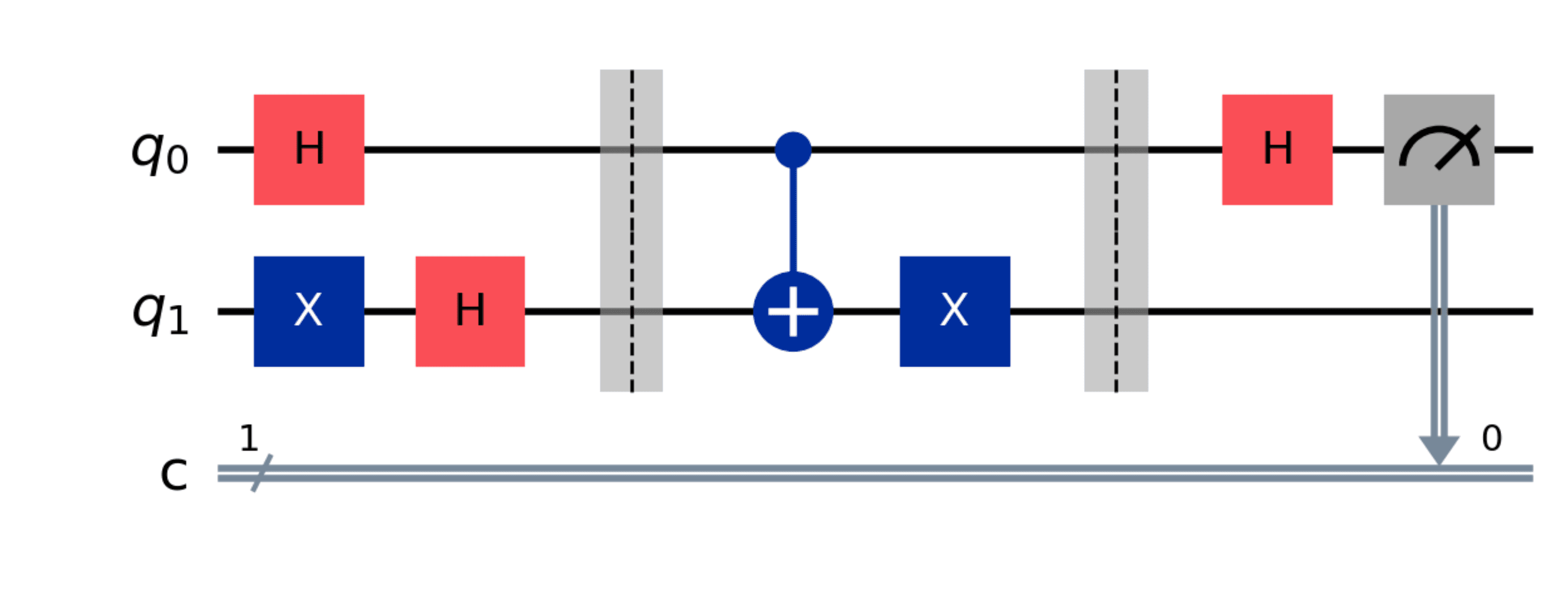
With that in place let's draw the circuit first for one of the oracles using:

deutsch_algorithm(balanced_not_x()).draw('mpl')

Deutsch's algorithm with a balanced not-x oracle

The main event will be running the algorithm on a real quantum computer. But before we do that, let's simulate the algorithm using Qiskit's Aer simulator.

for f in [
    constant_0,
    constant_1,
    balanced_x,
    balanced_not_x
]:
    qc = deutsch_algorithm(f())
    result = AerSimulator().run(qc, shots=100).result()
    counts = result.get_counts()
    print(f.__name__, counts)

which prints the simulated (ideal, if we were using a error-free quantum computer) results for each oracle:

constant_0 {'0': 100}
constant_1 {'0': 100}
balanced_x {'1': 100}
balanced_not_x {'1': 100}

As you can see, in the case of constant functions, the measurement is always 0 - in all of the 100 shots that we simulated.

And likewise in the case of balanced functions, the measurement is always 1.

Running the algorithm on a real quantum computer

Now let's verify those simulated results on a real quantum computer!

First, we need to grab a backend from IBM Quantum. There is a useful method to grab the least busy one so we don't have to wait too long:

backend = service.least_busy(operational=True, simulator=False, min_num_qubits=1)

Next, we create a quantum circuit with a given oracle function we want to test, for example a balanced one. We also transpile the circuit to the backend we're using.

qc = deutsch_algorithm(balanced_x())
qc_transpiled = transpile(qc, backend, optimization_level=2)

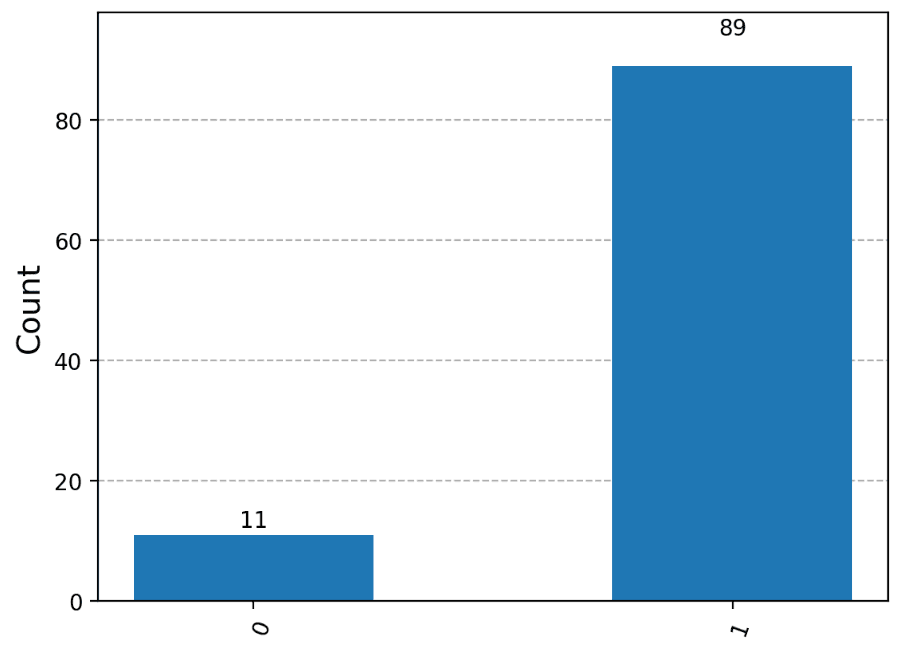
And finally, we run the circuit 100 times and plot the results.

sampler = Sampler(backend=backend)
qc_job = sampler.run([qc_transpiled], shots=100)
plot_histogram(qc_job.result()[0].data.c.get_counts())

This will show something like the following: Deutsch's algorithm results

Now this is not quite the same as the simulated results, but such is life in the NISQ era. Current quantum computers are too noisy to give us the exact results we expect. However the general trend is there: a balanced function will give us a 1 (in expectation).